Properties
Throughout this section, we assume \(\mathbf{K}\) and \(\mathbf{L}\) satisfy the sufficient conditions (3) and (4) respectively.
Relation between correlation and likelihood kernels
Considering the DPP defined by \(\mathbf{L} \succeq 0_N\), the associated correlation kernel \(\mathbf{K}\) (1) can be derived as
Considering the DPP defined by \(0_N \preceq \mathbf{K} \prec I_N\), the associated likelihood kernel \(\mathbf{L}\) (2) can be derived as
Important
Thus, except for correlation kernels \(\mathbf{K}\) with some eigenvalues equal to \(1\), both \(\mathbf{K}\) and \(\mathbf{L}\) are diagonalizable in the same basis
Note
For DPPs with projection correlation kernel \(\mathbf{K}\), the likelihood kernel \(\mathbf{L}\) cannot be computed via (7), since \(\mathbf{K}\) has at least one eigenvalue equal to \(1\) (\(\mathbf{K}^2=\mathbf{K}\)).
Nevertheless, if you recall that the number of points of a projection DPP, then its likelihood reads
from numpy.random import randn, rand
from scipy.linalg import qr
from dppy.finite_dpps import FiniteDPP

r, N = 4, 10
eig_vals = rand(r)  # 0< <1
eig_vecs, _ = qr(randn(N, r), mode='economic')

DPP = FiniteDPP('correlation', **{'K_eig_dec': (eig_vals, eig_vecs)})
DPP.compute_L()

# - L (likelihood) kernel computed via:
# - eig_L = eig_K/(1-eig_K)
# - U diag(eig_L) U.T
See also
Generic DPPs as mixtures of projection DPPs
Projection DPPs are the building blocks of the model in the sense that generic DPPs are mixtures of projection DPPs.
Important
Consider \(\mathcal{X} \sim \operatorname{DPP}(\mathbf{K})\) and write the spectral decomposition of the corresponding kernel as
Then, denote \(\mathcal{X}^B \sim \operatorname{DPP}(\mathbf{K}^B)\) with
where \(\mathcal{X}^B\) is obtained by first choosing \(B_1, \dots, B_N\) independently and then sampling from \(\operatorname{DPP}(\mathbf{K}^B)\) the DPP with orthogonal projection kernel \(\mathbf{K}^B\).
Finally, we have \(\mathcal{X} \overset{d}{=} \mathcal{X}^B\).
See also
Theorem 7 in [HKPVirag06]
Continuous case of Generic DPPs as mixtures of projection DPPs
Number of points
For projection DPPs, i.e., when \(\mathbf{K}\) is an orthogonal projection matrix, one can show that \(|\mathcal{X}|=\operatorname{rank}(\mathbf{K})=\operatorname{Trace}(\mathbf{K})\) almost surely (see, e.g., Lemma 17 of [HKPVirag06] or Lemma 2.7 of [KT12]).
In the general case, based on the fact that generic DPPs are mixtures of projection DPPs, we have
Note
From (9) it is clear that \(|\mathcal{X}|\leq \operatorname{rank}(\mathbf{K})=\operatorname{rank}(\mathbf{L})\).
Expectation
The expected size of a DPP with likelihood matrix \(\mathbf{L}\) is also related to the effective dimension \(d_{\text{eff}}(\mathbf{L}) = \operatorname{trace} (\mathbf{L}(\mathbf{L}+\mathbf{I})^{-1})= \operatorname{trace} \mathbf{K} = \mathbb{E}[|\mathcal{X}|]\) of \(\mathbf{L}\), a quantity with many applications in randomized numerical linear algebra and statistical learning theory (see e.g., [DerezinskiCV19]).
Variance
See also
Expectation and variance of Linear statistics.
import numpy as np
from scipy.linalg import qr
from dppy.finite_dpps import FiniteDPP

rng = np.random.RandomState(1)

r, N = 5, 10
eig_vals = rng.rand(r) # 0< <1
eig_vecs, _ = qr(rng.randn(N, r), mode='economic')

dpp_K = FiniteDPP('correlation', projection=False,
                **{'K_eig_dec': (eig_vals, eig_vecs)})

nb_samples = 2000
for _ in range(nb_samples):
    dpp_K.sample_exact(random_state=rng)

sizes = list(map(len, dpp_K.list_of_samples))
print('E[|X|]:\n emp={:.3f}, theo={:.3f}'
      .format(np.mean(sizes), np.sum(eig_vals)))
print('Var[|X|]:\n emp={:.3f}, theo={:.3f}'
      .format(np.var(sizes), np.sum(eig_vals*(1-eig_vals))))
E[|X|]:
 emp=1.581, theo=1.587
Var[|X|]:
 emp=0.795, theo=0.781
Special cases
When the correlation kernel \(\mathbf{K}\) (1) of \(\operatorname{DPP}(\mathbf{K})\) is an orthogonal projection kernel, i.e., \(\operatorname{DPP}(\mathbf{K})\) is a projection DPP, we have
(12)¶\[|\mathcal{X}| = \operatorname{rank}(\mathbf{K}) = \operatorname{trace}(\mathbf{K}), \quad \text{almost surely}.\]import numpy as np from scipy.linalg import qr from dppy.finite_dpps import FiniteDPP r, N = 4, 10 eig_vals = np.ones(r) eig_vecs, _ = qr(rng.randn(N, r), mode='economic') DPP = FiniteDPP('correlation', projection=True, **{'K_eig_dec': (eig_vals, eig_vecs)}) for _ in range(1000): DPP.sample_exact() sizes = list(map(len, DPP.list_of_samples)) # np.array(DPP.list_of_samples).shape = (1000, 4) assert([np.mean(sizes), np.var(sizes)] == [r, 0])
Important
Since \(|\mathcal{X}|=\operatorname{rank}(\mathbf{K})\) points, almost surely, the likelihood of the projection \(\operatorname{DPP}(\mathbf{K})\) reads
(13)¶\[\mathbb{P}[\mathcal{X}=S] = \det \mathbf{K}_S 1_{|S|=\operatorname{rank} \mathbf{K}}.\]In other words, the projection DPP having for correlation kernel the orthogonal projection matrix \(\mathbf{K}\) coincides with the k-DPP having likelihood kernel \(\mathbf{K}\) when \(k=\operatorname{rank}(\mathbf{K})\).
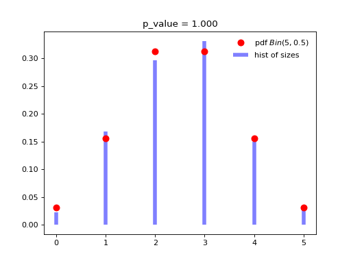
When the likelihood kernel \(\mathbf{L}\) of \(\operatorname{DPP}(\mathbf{L})\) (2) is an orthogonal projection kernel we have
(14)¶\[|\mathcal{X}| \sim \operatorname{Binomial}(\operatorname{rank}(\mathbf{L}), 1/2).\]import numpy as np from scipy.stats import binom, chisquare from scipy.linalg import qr import matplotlib.pyplot as plt from dppy.finite_dpps import FiniteDPP r, N = 5, 10 e_vals = np.ones(r) e_vecs, _ = qr(np.random.randn(N, r), mode='economic') dpp_L = FiniteDPP('likelihood', projection=True, **{'L_eig_dec': (e_vals, e_vecs)}) nb_samples = 1000 dpp_L.flush_samples for _ in range(nb_samples): dpp_L.sample_exact() sizes = list(map(len, dpp_L.list_of_samples)) p = 0.5 # binomial parameter rv = binom(r, p) fig, ax = plt.subplots(1, 1) x = np.arange(0, r + 1) pdf = rv.pmf(x) ax.plot(x, pdf, 'ro', ms=8, label=r'pdf $Bin({}, {})$'.format(r, p)) hist = np.histogram(sizes, bins=np.arange(0, r + 2), density=True)[0] ax.vlines(x, 0, hist, colors='b', lw=5, alpha=0.5, label='hist of sizes') ax.legend(loc='best', frameon=False) plt.title('p_value = {:.3f}'.format(chisquare(hist, pdf)[1])) plt.show()
(Source code, png, hires.png, pdf)

Fig. 5 Distribution of the numbe of points of \(\operatorname{DPP}(\mathbf{L})\) with orthogonal projection kernel \(\mathbf{L}\) with rank \(5\).
Geometrical insights
Kernels satisfying the sufficient conditions (3) and (4) can be expressed as
where each item is represented by a feature vector \(\phi_i\) (resp. \(\psi_i\)).
The geometrical view is then straightforward.
The inclusion probabilities read
\[\mathbb{P}[S\subset \mathcal{X}] = \det \mathbf{K}_S = \operatorname{Vol}^2 \{\phi_s\}_{s\in S}.\]The likelihood reads
\[\mathbb{P}[\mathcal{X} = S] \propto \det \mathbf{L}_S = \operatorname{Vol}^2 \{\psi_s\}_{s\in S}.\]
That is to say, DPPs favor subsets \(S\) whose corresponding feature vectors span a large volume i.e. DPPs sample softened orthogonal bases.
Diversity
The determinantal structure of DPPs encodes the notion of diversity. Deriving the pair inclusion probability, also called the 2-point correlation function using (1), we obtain
so that, the larger \(|\mathbf{K}_{i j}|\) less likely items \(i\) and \(j\) co-occur. If \(K_{ij}\) models the similarity between items \(i\) and \(j\), DPPs are thus random diverse sets of elements.
Conditioning
Like many other statistics of DPPs, the conditional probabilities can be expressed my means of a determinant and involve the correlation kernel \(\mathbf{K}\) (1).
For any disjoint subsets \(S, T \subset [N]\), i.e., such that \(S\cap T = \emptyset\) we have
See also
Propositions 3 and 5 of [Pou19] for the proofs
Equations (15) and (15) are key to derive the Cholesky-based exact sampler which makes use of the chain rule on sets.