Multivariate Jacobi ensemble

Important

For the details please refer to:

1. the extensive documentation of MultivariateJacobiOPE below

2. the associated Jupyter notebook which showcases MultivariateJacobiOPE

3. our NeurIPS‘19 paper [GBV19] On two ways to use determinantal point processes for Monte Carlo integration

4. our ICML‘19 workshop paper

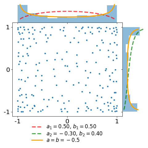
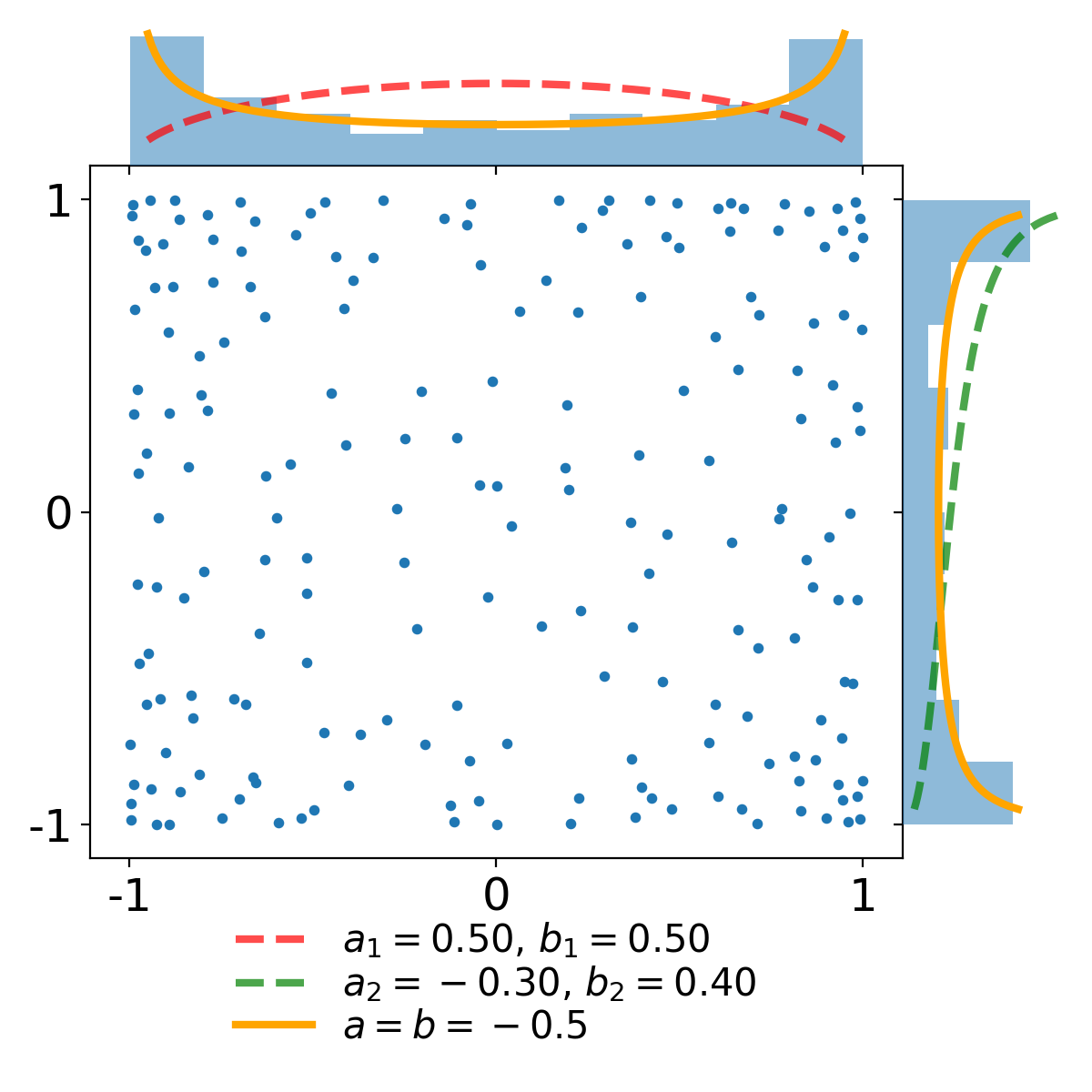
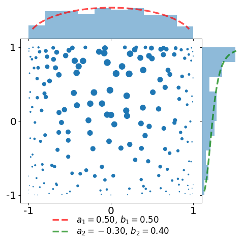
The figures below display a sample of a \(d=2\) dimensional Jacobi ensemble MultivariateJacobiOPE with \(N=200\) points. The red and green dashed curves correspond to the normalized base densities proportional to \((1-x)^{a_1} (1+x)^{b_1}\) and \((1-y)^{a_2} (1+y)^{b_2}\), respectively.

import numpy as np
import matplotlib.pyplot as plt
from dppy.multivariate_jacobi_ope import MultivariateJacobiOPE

# The .plot() method outputs smtg only in dimension d=1 or 2

# Number of points / dimension
N, d = 200, 2
# Jacobi parameters in [-0.5, 0.5]^{d x 2}
jac_params = np.array([[0.5, 0.5],
                       [-0.3, 0.4]])

dpp = MultivariateJacobiOPE(N, jac_params)

# Get an exact sample
sampl = dpp.sample()

# Display
# the cloud of points
# the base probability densities
# the marginal empirical histograms
dpp.plot(sample=sampl, weighted=False)
plt.tight_layout()

# Attach a weight 1/K(x,x) to each of the points
dpp.plot(sample=sampl, weighted=True)
plt.tight_layout()

(Source code)

Fig. 42 (png, hires.png, pdf)

Fig. 43 (png, hires.png, pdf)

• In the first plot, observe that the empirical marginal density converges to the arcsine density \(\frac{1}{\pi\sqrt{1-x^2}}\), displayed in orange.

• In the second plot, we take the same sample and attach a weight \(\frac{1}{K(x,x)}\) to each of the points. This illustrates the choice of the weights defining the estimator of [BH16] as a proxy for the reference measure.

---

Implementation of the class MultivariateJacobiOPE used in [GBV19] for Monte Carlo with Determinantal Point Processes

It has 3 main methods:

• sample() to generate samples

• K() to evaluate the corresponding projection kernel

• plot() to display 1D or 2D samples

class dppy.multivariate_jacobi_ope.MultivariateJacobiOPE(N, jacobi_params)

Bases: object

Multivariate Jacobi Orthogonal Polynomial Ensemble used in [GBV19] for Monte Carlo with Determinantal Point Processes

This corresponds to a continuous multivariate projection DPP with state space \([-1, 1]^d\) with respect to

• reference measure \(\mu(dx) = w(x) dx\) (see also eval_w()), where

  \[w(x) = \prod_{i=1}^{d} (1-x_i)^{a_i} (1+x_i)^{b_i}\]

• kernel \(K\) (see also K())

  \[K(x, y) = \sum_{\mathfrak{b}(k)=0}^{N-1} P_{k}(x) P_{k}(y) = \Phi(x)^{\top} \Phi(y)\]

  where

  • \(k \in \mathbb{N}^d\) is a multi-index ordered according to the ordering \(\mathfrak{b}\) (see compute_ordering())

  • \(P_{k}(x) = \prod_{i=1}^d P_{k_i}^{(a_i, b_i)}(x_i)\) is the product of orthonormal Jacobi polynomials

    \[\int_{-1}^{1} P_{k}^{(a_i,b_i)}(u) P_{\ell}^{(a_i,b_i)}(u) (1-u)^{a_i} (1+u)^{b_i} d u = \delta_{k\ell}\]

    so that \((P_{k})\) are orthonormal w.r.t \(\mu(dx)\)

  • \(\Phi(x) = \left(P_{\mathfrak{b}^{-1}(0)}(x), \dots, P_{\mathfrak{b}^{-1}(N-1)}(x) \right)^{\top}\)

Parameters

• N (int) – Number of points \(N \geq 1\)

• jacobi_params (array_like) – Jacobi parameters \([(a_i, b_i)]_{i=1}^d\) The number of rows \(d\) prescribes the ambient dimension of the points i.e. \(x_{1}, \dots, x_{N} \in [-1, 1]^d\). - when \(d=1\), \(a_1, b_1 > -1\) - when \(d \geq 2\), \(|a_i|, |b_i| \leq \frac{1}{2}\)

See also

• Multivariate Jacobi ensemble

• when \(d=1\), the univariate Jacobi ensemble is sampled by computing the eigenvalues of a properly randomized tridiagonal matrix of [KN04]

• [BH16] initiated the use of the multivariate Jacobi ensemble for Monte Carlo integration. In particular, they proved CLT with variance decay of order \(N^{-(1+1/d)}\) which is faster that the \(N^{-1}\) rate of vanilla Monte Carlo where the points are drawn i.i.d. from the base measure.

K(X, Y=None, eval_pointwise=False)

Evalute \(\left(K(x, y)\right)_{x\in X, y\in Y}\) if eval_pointwise=False or \(\left(K(x, y)\right)_{(x, y)\in (X, Y)}\) otherwise

\[K(x, y) = \sum_{\mathfrak{b}(k)=0}^{N-1} P_{k}(x) P_{k}(y) = \phi(x)^{\top} \phi(y)\]

where

• \(k \in \mathbb{N}^d\) is a multi-index ordered according to the ordering \(\mathfrak{b}\), compute_ordering()

• \(P_{k}(x) = \prod_{i=1}^d P_{k_i}^{(a_i, b_i)}(x_i)\) is the product of orthonormal Jacobi polynomials

  \[\int_{-1}^{1} P_{k}^{(a_i,b_i)}(u) P_{\ell}^{(a_i,b_i)}(u) (1-u)^{a_i} (1+u)^{b_i} d u = \delta_{k\ell}\]

  so that \((P_{k})\) are orthonormal w.r.t \(\mu(dx)\)

• \(\Phi(x) = \left(P_{\mathfrak{b}^{-1}(0)}(x), \dots, P_{\mathfrak{b}^{-1}(N-1)}(x) \right)\), see eval_multiD_polynomials()

Parameters

• X (array_like) – \(M\times d\) array of \(M\) points \(\in [-1, 1]^d\)

• Y (array_like (default None)) – \(M'\times d\) array of \(M'\) points \(\in [-1, 1]^d\)

• eval_pointwise (bool (default False)) – sets pointwise evaluation of the kernel, if True, \(X\) and \(Y\) must have the same shape, see Returns

Returns

If eval_pointwise=False (default), evaluate the kernel matrix

\[\left(K(x, y)\right)_{x\in X, y\in Y}\]

If eval_pointwise=True kernel matrix Pointwise evaluation of \(K\) as depicted in the following pseudo code output

• if Y is None

  • \(\left(K(x, y)\right)_{x\in X, y\in X}\) if eval_pointwise=False

  • \(\left(K(x, x)\right)_{x\in X}\) if eval_pointwise=True

• otherwise

  • \(\left(K(x, y)\right)_{x\in X, y\in Y}\) if eval_pointwise=False

  • \(\left(K(x, y)\right)_{(x, y)\in (X, Y)}\) if eval_pointwise=True (in this case X and Y should have the same shape)

Return type

array_like

See also

eval_multiD_polynomials()

eval_multiD_polynomials(X)

Evaluate

\[\begin{split}\mathbf{\Phi}(X) := \begin{pmatrix} \Phi(x_1)^{\top}\\ \vdots\\ \Phi(x_M)^{\top} \end{pmatrix}\end{split}\]

where \(\Phi(x) = \left(P_{\mathfrak{b}^{-1}(0)}(x), \dots, P_{\mathfrak{b}^{-1}(N-1)}(x) \right)^{\top}\) such that \(K(x, y) = \Phi(x)^{\top} \Phi(y)\). Recall that \(\mathfrak{b}\) denotes the ordering chosen to order multi-indices \(k\in \mathbb{N}^d\).

This is done by evaluating each of the three-term recurrence relations satisfied by each univariate orthogonal Jacobi polynomial, using the dedicated see also SciPy scipy.special.eval_jacobi() satistified by the respective univariate Jacobi polynomials \(P_{k_i}^{(a_i, b_i)}(x_i)\). Then we use the slicing feature of the Python language to compute \(\Phi(x)=\left(P_{k}(x) = \prod_{i=1}^d P_{k_i}^{(a_i, b_i)}(x_i)\right)_{k=\mathfrak{b}^{-1}(0), \dots, \mathfrak{b}^{-1}(N-1)}^{\top}\)

Parameters

X (array_like) – \(M\times d\) array of \(M\) points \(\in [-1, 1]^d\)

Returns

\(\mathbf{\Phi}(X)\) - \(M\times N\) array

Return type

array_like

See also

• evaluation of the kernel K()

eval_w(X)

Evaluate \(w(x) = \prod_{i=1}^{d} (1-x_i)^{a_i} (1+x_i)^{b_i}\) which corresponds to the density of the base measure \(\mu(dx) = w(x) dx\)

Parameters

X (array_like) – \(M\times d\) array of \(M\) points \(\in [-1, 1]^d\)

Returns

\(w(x) = \prod_{i=1}^{d} (1-x_i)^{a_i} (1+x_i)^{b_i}\)

Return type

array_like

sample(nb_trials_max=10000, random_state=None, tridiag_1D=True)

Use the chain rule [HKPVirag06] (Algorithm 18) to sample \(\left(x_{1}, \dots, x_{N} \right)\) with density

\[\begin{split}& \frac{1}{N!} \left(K(x_n,x_p)\right)_{n,p=1}^{N} \prod_{n=1}^{N} w(x_n)\\ &= \frac{1}{N} K(x_1,x_1) w(x_1) \prod_{n=2}^{N} \frac{ K(x_n,x_n) - K(x_n,x_{1:n-1}) \left[\left(K(x_k,x_l)\right)_{k,l=1}^{n-1}\right]^{-1} K(x_{1:n-1},x_n) }{N-(n-1)} w(x_n)\\ &= \frac{\| \Phi(x) \|^2}{N} \omega(x_1) d x_1 \prod_{n=2}^{N} \frac{\operatorname{distance}^2(\Phi(x_n), \operatorname{span}\{\Phi(x_p)\}_{p=1}^{n-1})} {N-(n-1)} \omega(x_n) d x_n\end{split}\]

The order in which the points were sampled can be forgotten to obtain a valid sample of the corresponding DPP

• \(x_1 \sim \frac{1}{N} K(x,x) w(x)\) using sample_chain_rule_proposal()

• \(x_n | Y = \left\{ x_{1}, \dots, x_{n-1} \right\}\), is sampled using rejection sampling with proposal density \(\frac{1}{N} K(x,x) w(x)\) and rejection bound frac{N}{N-(n-1)}

  \[\frac{1}{N-(n-1)} [K(x,x) - K(x, Y) K_Y^{-1} K(Y, x)] w(x) \leq \frac{N}{N-(n-1)} \frac{1}{N} K(x,x) w(x)\]

Note

Using the gram structure \(K(x, y) = \Phi(x)^{\top} \Phi(y)\) the numerator of the successive conditionals reads

\[\begin{split}K(x, x) - K(x, Y) K(Y, Y)^{-1} K(Y, x) &= \operatorname{distance}^2(\Phi(x_n), \operatorname{span}\{\Phi(x_p)\}_{p=1}^{n-1})\\ &= \left\| (I - \Pi_{\operatorname{span}\{\Phi(x_p)\}_{p=1}^{n-1}} \phi(x)\right\|^2\end{split}\]

which can be computed simply in a vectorized way. The overall procedure is akin to a sequential Gram-Schmidt orthogonalization of \(\Phi(x_{1}), \dots, \Phi(x_{N})\).

See also

• Projection DPPs: the chain rule

• sample_chain_rule_proposal()

sample_chain_rule_proposal(nb_trials_max=10000, random_state=None)

Use a rejection sampling mechanism to sample

\[\frac{1}{N} K(x, x) w(x) dx = \frac{1}{N} \sum_{\mathfrak{b}(k)=0}^{N-1} \left( \frac{P_k(x)}{\left\| P_k \right\|} \right)^2 w(x)\]

with proposal distribution

\[w_{eq}(x) d x = \prod_{i=1}^{d} \frac{1}{\pi\sqrt{1-(x_i)^2}} d x_i\]

Since the target density is a mixture, we can sample from it by

1. Select a multi-index \(k\) uniformly at random in \(\left\{ \mathfrak{b}^{-1}(0), \dots, \mathfrak{b}^{-1}(N-1) \right\}\)

2. Sample from \(\left( \frac{P_k(x)}{\left\| P_k \right\|} \right)^2 w(x) dx\) with proposal \(w_{eq}(x) d x\).

   The acceptance ratio writes

   \[\frac{ \left( \frac{P_k(x)}{\left\| P_k \right\|} \right)^2 w(x)} {w_{eq}(x)} = \prod_{i=1}^{d} \pi \left( \frac{P_{k_i}^{(a_i, b_i)}(x)} {\left\| P_{k_i}^{(a_i, b_i)} \right\|} \right)^2 (1-x_i)^{a_i+\frac{1}{2}} (1+x_i)^{b_i+\frac{1}{2}} \leq C_{k}\]

   which can be bounded using the result of [Gau09] on Jacobi polynomials.

   Note

   Each of the rejection constant \(C_{k}\) is computed at initialization of the MultivariateJacobiOPE object using compute_rejection_bounds()

Returns

A sample \(x\in[-1,1]^d\) with probability distribution \(\frac{1}{N} K(x,x) w(x)\)

Return type

array_like

See also

• compute_rejection_bounds()

• sample()

dppy.multivariate_jacobi_ope.compute_degrees_1D_polynomials(max_degrees)

deg[i, j] = i if i <= max_degrees[j] else 0

dppy.multivariate_jacobi_ope.compute_norms_1D_polynomials(jacobi_params, deg_max)

Compute the square norms \(\|P_{k}^{(a_i,b_i)}\|^2\) of each (univariate) orthogoanl Jacobi polynomial for \(k=0\) to deg_max and \(a_i, b_i =\) jacobi_params[i, :] Recall that the Jacobi polynomials \(\left( P_{k}^{(a_i,b_i)} \right)\) are orthogonal w.r.t. \((1-u)^{a_i} (1+u)^{b_i} du\).

\[\begin{split}\|P_{k}^{(a_i,b_i)}\|^2 &= \int_{-1}^{1} \left( P_{k}^{(a_i,b_i)}(u) \right)^2 (1-u)^{a_i} (1+u)^{b_i} d u\\ &= \frac{2^{a_i+b_i+1}} {2k+a_i+b_i+1} \frac{\Gamma(k+a_i+1)\Gamma(k+b_i+1)} {\Gamma(k+a_i+b_i+1)n!}\end{split}\]

Parameters

• jacobi_params (array_like) – Jacobi parameters \([(a_i, b_i)]_{i=1}^d \in [-\frac{1}{2}, \frac{1}{2}]^{d \times 2}\) The number of rows \(d\) prescribes the ambient dimension of the points i.e. \(x_{1}, \dots, x_{N} \in [-1, 1]^d\)

• deg_max (int) – Maximal degree of 1D Jacobi polynomials

Returns

Array of size deg_max + 1 \(\times d\) with entry \(k,i\) given by \(\|P_{k}^{(a_i,b_i)}\|^2\)

Return type

array_like

See also

• Wikipedia Jacobi polynomials

• compute_ordering()

dppy.multivariate_jacobi_ope.compute_ordering(N, d)

Compute the ordering of the multi-indices \(\in\mathbb{N}^d\) defining the order between the multivariate monomials as described in Section 2.1.3 of [BH16].

Parameters

• N (int) – Number of polynomials \((P_k)\) considered to build the kernel K() (number of points of the corresponding MultivariateJacobiOPE)

• d (int) – Size of the multi-indices \(k\in \mathbb{N}^d\) characterizing the _degree_ of \(P_k\) (ambient dimension of the points x_{1}, dots, x_{N} in [-1, 1]^d)

Returns

Array of size \(N\times d\) containing the first \(N\) multi-indices \(\in\mathbb{N}^d\) in the order prescribed by the ordering \(\mathfrak{b}\) [BH16] Section 2.1.3

Return type

array_like

For instance, for \(N=12, d=2\)

[(0, 0), (0, 1), (1, 0), (1, 1), (0, 2), (1, 2), (2, 0), (2, 1), (2, 2), (0, 3), (1, 3), (2, 3)]

See also

• [BH16] Section 2.1.3

dppy.multivariate_jacobi_ope.compute_rejection_bounds(jacobi_params, ordering, log_scale=True)

Compute the rejection constants for the acceptance/rejection mechanism used in sample_chain_rule_proposal() to sample

\[\frac{1}{N} K(x, x) w(x) dx = \frac{1}{N} \sum_{\mathfrak{b}(k)=0}^{N-1} \left( \frac{P_k(x)}{\left\| P_k \right\|} \right)^2 w(x)\]

with proposal distribution

\[w_{eq}(x) d x = \prod_{i=1}^{d} \frac{1}{\pi\sqrt{1-(x_i)^2}} d x_i\]

To get a sample:

1. Draw a multi-index \(k\) uniformly at random in \(\left\{ \mathfrak{b}^{-1}(0), \dots, \mathfrak{b}^{-1}(N-1) \right\}\)

2. Sample from \(P_k(x)^2 w(x) dx\) with proposal \(w_{eq}(x) d x\).

   The acceptance ratio writes

   \[\frac{\left( \frac{P_k(x)}{\left\| P_k \right\|} \right)^2 w(x)} {w_{eq}(x)} = \prod_{i=1}^{d} \pi \left( \frac{P_{k_i}^{(a_i, b_i)}(x)} {\left\| P_{k_i}^{(a_i, b_i)} \right\|} \right)^2 (1-x_i)^{a_i+\frac{1}{2}} (1+x_i)^{b_i+\frac{1}{2}} \leq C_k\]

   • For \(k_i>0\) we use a result on Jacobi polynomials given by, e.g., [Gau09], for \(\quad|a|,|b| \leq \frac{1}{2}\)

   \[\begin{split}& \pi (1-u)^{a+\frac{1}{2}} (1+u)^{b+\frac{1}{2}} \left( \frac{P_{n}^{(a, b)}(u)} {\left\| P_{n}^{(a, b)} \right\|} \right)^2\\ &\leq \frac{2} {n!(n+(a+b+1) / 2)^{2 \max(a,b)}} \frac{\Gamma(n+a+b+1) \Gamma(n+\max(a,b)+1)} {\Gamma(n+\min(a,b)+1)}\end{split}\]

   • For \(k_i=0\), we use less involved properties of the Jacobi polynomials:

     • \(P_{0}^{(a, b)} = 1\)

     • \(\|P_{0}^{(a, b)}\|^2 = 2^{a+b+1} \operatorname{B}(a+1,b+1)\)

     • \(m = \frac{b-a}{a+b+1}\) is the mode of \((1-u)^{a+\frac{1}{2}} (1+u)^{b+\frac{1}{2}}\) (valid since \(a+\frac{1}{2}, b+\frac{1}{2} > 0\))

     So that,

     \[\begin{split} \pi (1-u)^{a+\frac{1}{2}} (1+u)^{b+\frac{1}{2}} \left(\frac{P_{0}^{(a, b)}(u)} {\|P_{0}^{(a, b)}\|}\right)^{2} &= \frac {\pi (1-u)^{a+\frac{1}{2}} (1+u)^{b+\frac{1}{2}}} {\|P_{0}^{(a, b)}\|^2} \\ &\leq \frac {\pi (1-m)^{a+\frac{1}{2}} (1+m)^{b+\frac{1}{2}}} {2^{a+b+1} \operatorname{B}(a+1,b+1)}\end{split}\]

Parameters

• jacobi_params (array_like) –

  Jacobi parameters \([(a_i, b_i)]_{i=1}^d \in [-\frac{1}{2}, \frac{1}{2}]^{d \times 2}\).

  The number of rows \(d\) prescribes the ambient dimension of the points i.e. \(x_{1}, \dots, x_{N} \in [-1, 1]^d\)

• ordering (array_like) –

  Ordering of the multi-indices \(\in\mathbb{N}^d\) defining the order between the multivariate monomials (see also compute_ordering())

  • the number of rows corresponds to the number \(N\) of monomials considered.

  • the number of columns \(=d\)

• log_scale (bool) – If True, the rejection bound is computed using the logarithmic versions betaln, gammaln of beta and gamma functions to avoid overflows

Returns

The rejection bounds \(C_{k}\) for \(k = \mathfrak{b}^{-1}(0), \dots, \mathfrak{b}^{-1}(N-1)\)

Return type

array_like

See also

• [Gau09] for the domination when \(k_i > 0\)

• compute_poly1D_norms()