Banded matrix models
Computing the eigenvalues of a full \(N\times N\) random matrix is \(\mathcal{O}(N^3)\), and can thus become prohibitive for large \(N\). A way to circumvent the problem is to adopt the equivalent banded models i.e. diagonalize banded matrices.
The first tridiagonal models for the Hermite Ensemble and Laguerre Ensemble were revealed by [DE02], who left the Jacobi Ensemble as an open question, addressed by [KN04]. Such tridiagonal formulations made sampling possible at cost \(\mathcal{O}(N^2)\) but also unlocked sampling for generic \(\beta>0\)!
Note that [KN04] also derived a quindiagonal model for the Circular Ensemble.
Hermite Ensemble
Take for reference measure \(\mu=\mathcal{N}(\mu, \sigma)\)
Note
Recall that from the definition in (33)
The equivalent tridiagonal model reads
with
To recover the full matrix model for Hermite Ensemble, recall that \(\Gamma(\frac{k}{2}, 2)\equiv \chi_k^2\) and take
That is to say,
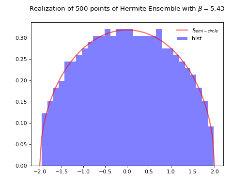
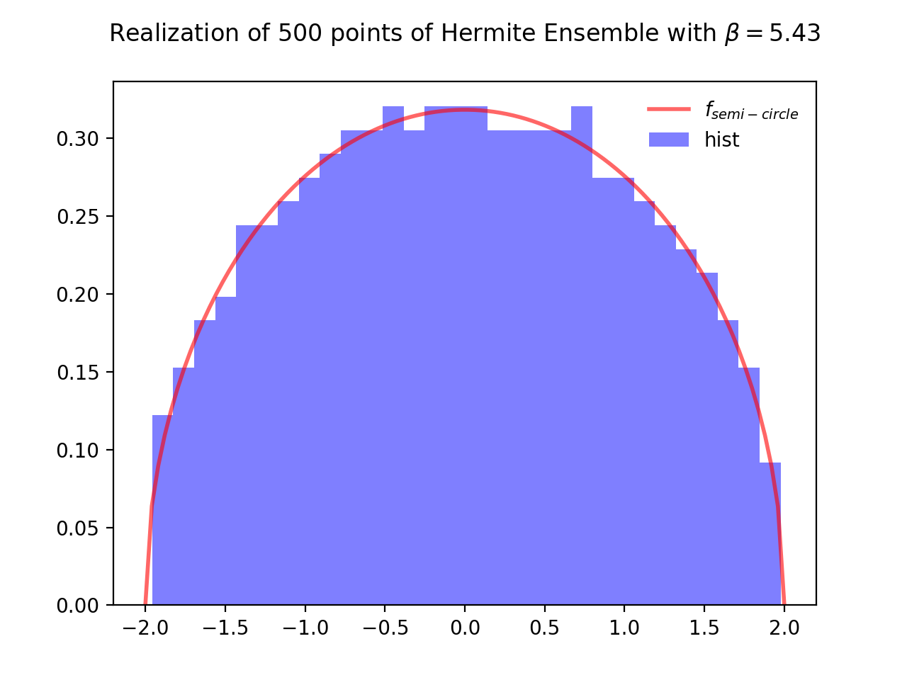
from dppy.beta_ensembles import HermiteEnsemble


hermite = HermiteEnsemble(beta=5.43)  # beta can be >=0, default beta=2
# Reference measure is N(mu, sigma^2)
hermite.sample_banded_model(loc=0.0, scale=1.0, size_N=500)
# hermite.plot(normalization=True)
hermite.hist(normalization=True)
(Source code, png, hires.png, pdf)

Fig. 26 Tridiagonal matrix model for the Hermite ensemble
See also
[DE02] II-C
Full matrix model for Hermite ensemble
HermiteEnsemblein API
Laguerre Ensemble
Take for reference measure \(\mu=\Gamma(k,\theta)\)
Note
Recall that from the definition in (33)
The equivalent tridiagonal model reads
with
To recover the full matrix model for Laguerre Ensemble, recall that \(\Gamma(\frac{k}{2}, 2)\equiv \chi_k^2\) and take
That is to say,
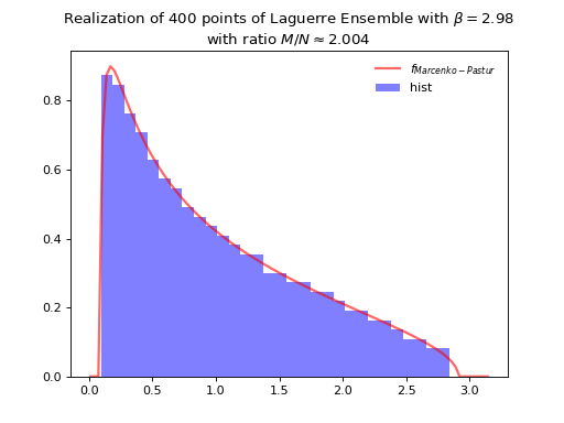
from dppy.beta_ensembles import LaguerreEnsemble


laguerre = LaguerreEnsemble(beta=2.98)  # beta can be >=0, default beta=2
# Reference measure is Gamma(k, theta)
laguerre.sample_banded_model(shape=600, scale=2.0, size_N=400)
# laguerre.plot(normalization=True)
laguerre.hist(normalization=True)
(Source code, png, hires.png, pdf)

Fig. 28 Tridiagonal matrix model for the Laguerre ensemble
See also
[DE02] III-B
Full matrix model for Laguerre ensemble
LaguerreEnsemblein API
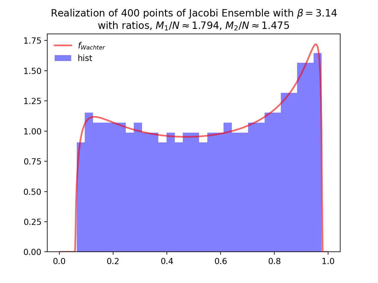
Jacobi Ensemble
Take for reference measure \(\mu=\operatorname{Beta}(a,b)\)
Note
Recall that from the definition in (33)
The equivalent tridiagonal model reads
with
To recover the full matrix model for Laguerre Ensemble, recall that \(\Gamma(\frac{k}{2}, 2)\equiv \chi_k^2\) and take
That is to say,
from dppy.beta_ensembles import JacobiEnsemble


jacobi = JacobiEnsemble(beta=3.14)  # beta can be >=0, default beta=2
# Reference measure is Beta(a,b)
jacobi.sample_banded_model(a=500, b=300, size_N=400)
# jacobi.plot(normalization=True)
jacobi.hist(normalization=True)
(Source code, png, hires.png, pdf)

Fig. 30 Tridiagonal matrix model for the Jacobi ensemble
See also
[KN04] Theorem 2
Full matrix model for Jacobi ensemble
JacobiEnsemblein APIMultivariateJacobiOPEin API
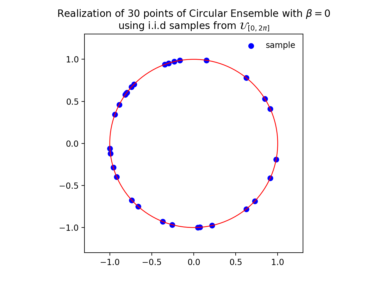
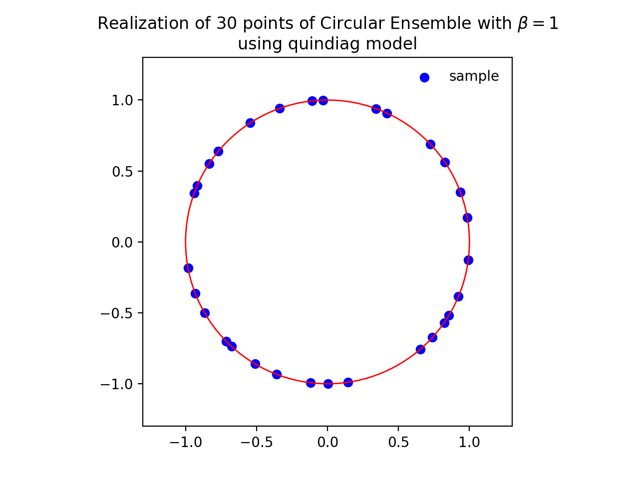
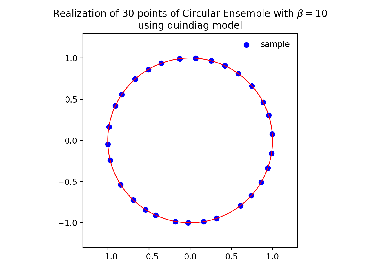
Circular Ensemble
Note
Recall that from the definition in (33)
Important
Consider the distribution \(\Theta_{\nu}\) that for integers \(\nu\geq2\) is defined as follows:
Draw \(v\) uniformly at random from the unit sphere \(\mathbb{S}^{\nu} \in \mathbb{R}^{\nu+1}\), then \(v_1 + iv_2\sim \Theta_{\nu}\)
Now, given \(\beta\in \mathbb{N}^*\), let
\(\alpha_k\sim \Theta_{\beta(N-k-1)+1}\) independent variables
for \(0\leq k\leq N-1\) set \(\rho_k = \sqrt{1-|\alpha_k|^2}\).
Then, the equivalent quindiagonal model corresponds to the eigenvalues of either \(LM\) or \(ML\) with
and where
Hint
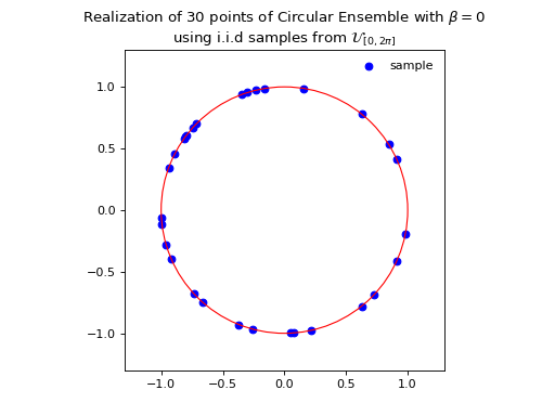
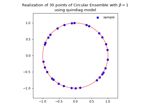
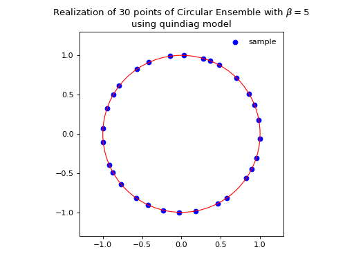
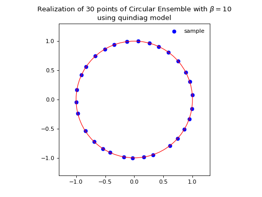
The effect of increasing the \(\beta\) parameter can be nicely visualized on this Circular Ensemble. Viewing \(\beta\) as the inverse temperature, the configuration of the eigenvalues crystallizes with \(\beta\), see the figure below.
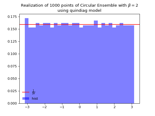
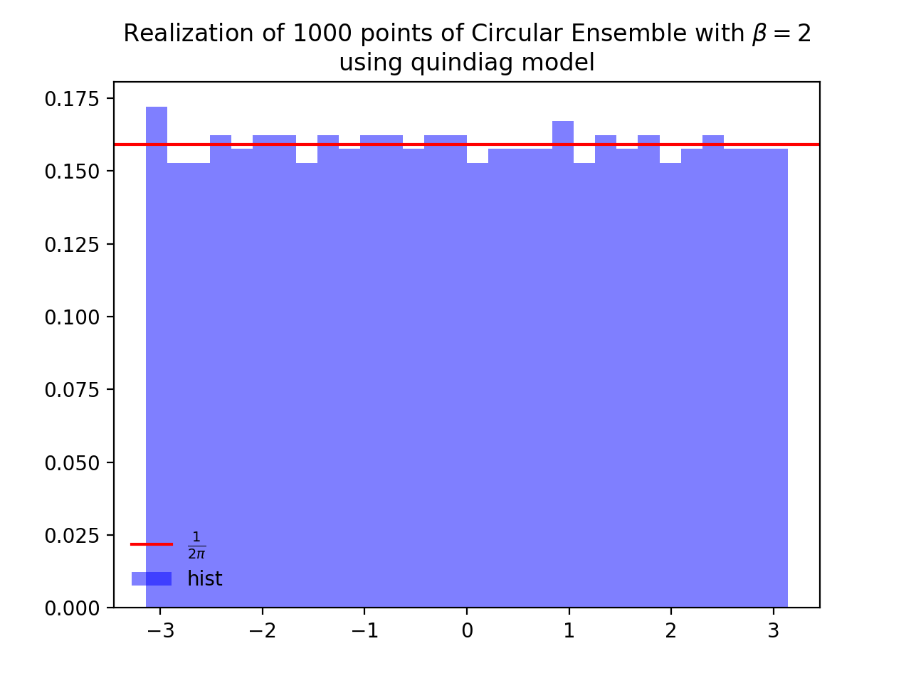
from dppy.beta_ensembles import CircularEnsemble

circular = CircularEnsemble(beta=2)  # beta must be >=0 integer, default beta=2

# See the cristallization of the configuration as beta increases
for b in [0, 1, 5, 10]:

    circular.beta = b
    circular.sample_banded_model(size_N=30)
    circular.plot()

circular.beta = 2
circular.sample_banded_model(size_N=1000)
circular.hist()
See also
[KN04] Theorem 1
Full matrix model for Circular ensemble
CircularEnsemblein API