Full matrix models
For specific reference measures the \(\beta = 1, 2, 4\) cases are very singular in the sense that the corresponding ensembles coincide with the eigenvalues of random matrices.
This is a highway for sampling exactly such ensembles in \(\mathcal{O}(N^3)\)!
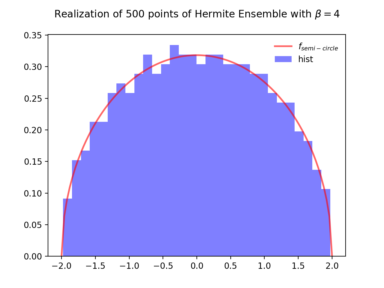
Hermite Ensemble
Take for reference measure \(\mu=\mathcal{N}(0, 2)\), the pdf of the corresponding \(\beta\)-Ensemble reads
Hint
The Hermite ensemble (whose name comes from the fact that Hermite polynomials are orthogonal w.r.t the Gaussian distribution) refers to the eigenvalue distribution of random matrices formed by i.i.d. Gaussian vectors.
\(\beta=1\)
\(\beta=2\)
\(\beta=4\)
Normalization \(\sqrt{\beta N}\) to concentrate as the semi-circle law.
from dppy.beta_ensembles import HermiteEnsemble


hermite = HermiteEnsemble(beta=4)  # beta in {0,1,2,4}, default beta=2
hermite.sample_full_model(size_N=500)
# hermite.plot(normalization=True)
hermite.hist(normalization=True)

# To compare with the sampling speed of the tridiagonal model simply use
# hermite.sample_banded_model(size_N=500)
(Source code, png, hires.png, pdf)

Fig. 8 Full matrix model for the Hermite ensemble
See also
Banded matrix model for Hermite ensemble
HermiteEnsemblein API
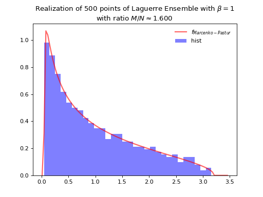
Laguerre Ensemble
Take for reference measure \(\mu=\Gamma\left(\frac{\beta}{2}(M-N+1), 2\right)=\chi_{\beta(M-N+1)}^2\), the pdf of the corresponding \(\beta\)-Ensemble reads
Hint
The Laguerre ensemble (whose name comes from the fact that Laguerre polynomials are orthogonal w.r.t the Gamma distribution) refers to the eigenvalue distribution of empirical covariance matrices of i.i.d. Gaussian vectors.
\(\beta=1\)
\(\beta=2\)
\(\beta=4\)
Normalization \(\beta M\) to concentrate as Marcenko-Pastur law.
where
from dppy.beta_ensembles import LaguerreEnsemble


laguerre = LaguerreEnsemble(beta=1)  # beta in {0,1,2,4}, default beta=2
laguerre.sample_full_model(size_N=500, size_M=800)  # M >= N
# laguerre.plot(normalization=True)
laguerre.hist(normalization=True)

# To compare with the sampling speed of the tridiagonal model simply use
# laguerre.sample_banded_model(size_N=500, size_M=800)
(Source code, png, hires.png, pdf)

Fig. 10 Full matrix model for the Laguerre ensemble
See also
Banded matrix model for Laguerre ensemble
LaguerreEnsemblein API
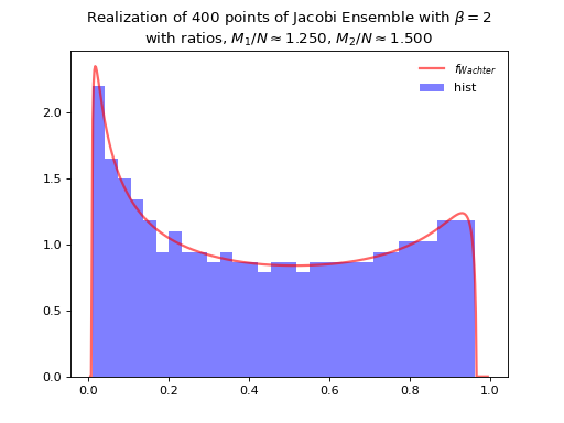
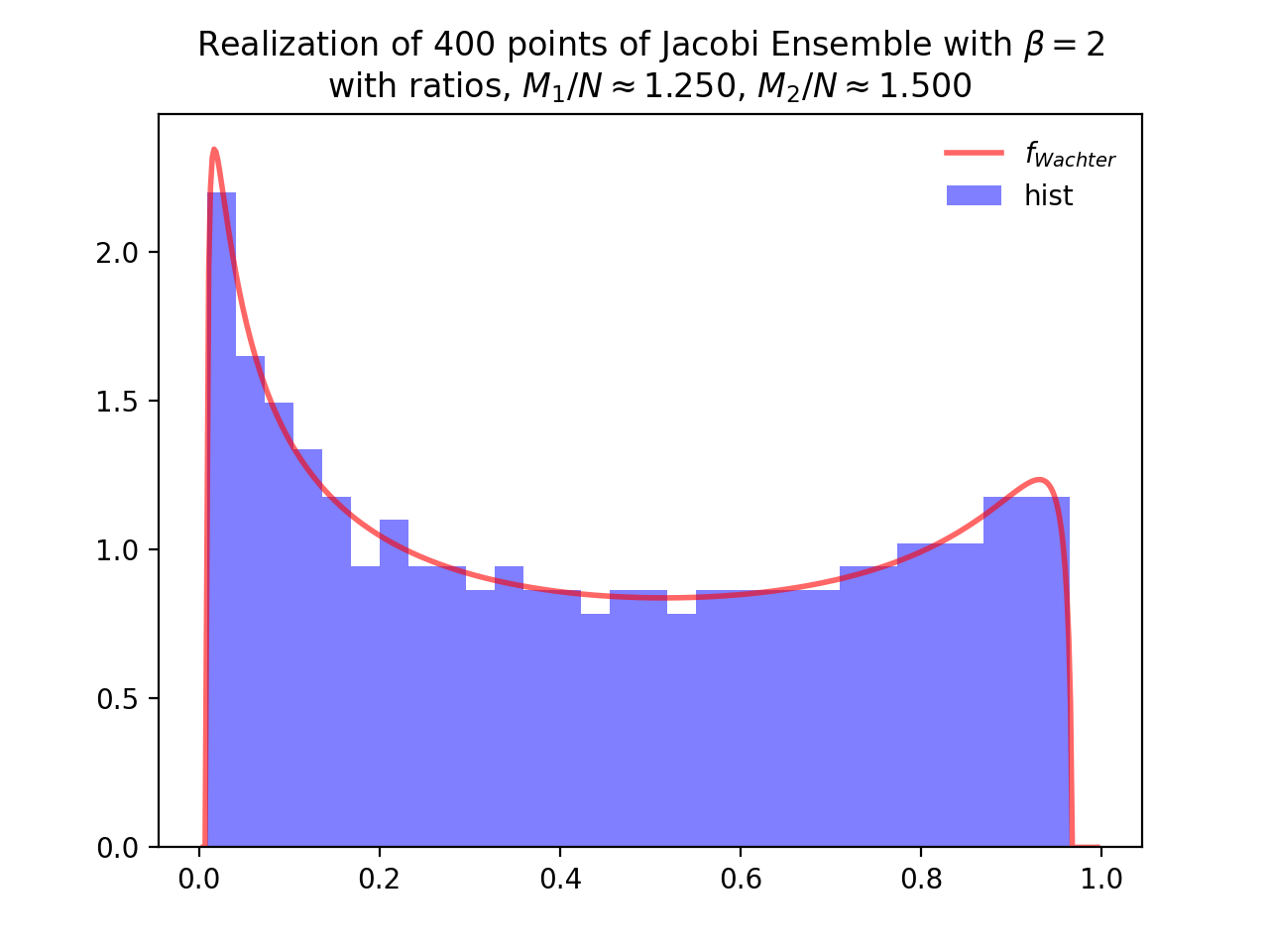
Jacobi Ensemble
Take for reference measure \(\mu=\operatorname{Beta}\left(\frac{\beta}{2}(M_1-N+1), \frac{\beta}{2}(M_2-N+1)\right)\), the pdf of the corresponding \(\beta\)-Ensemble reads
Hint
The Jacobi ensemble (whose name comes from the fact that Jacobi polynomials are orthogonal w.r.t the Beta distribution) is associated with the multivariate analysis of variance (MANOVA) model.
\(\beta=1\)
\(\beta=2\)
\(\beta=4\)
Concentrates as Wachter law
where
itself tending to the arcsine law in the limit.
from dppy.beta_ensembles import JacobiEnsemble


jacobi = JacobiEnsemble(beta=2)  # beta must be in {0,1,2,4}, default beta=2
jacobi.sample_full_model(size_N=400, size_M1=500, size_M2=600)  # M_1, M_2 >= N
# jacobi.plot(normalization=True)
jacobi.hist(normalization=True)

# To compare with the sampling speed of the triadiagonal model simply use
# jacobi.sample_banded_model(size_N=400, size_M1=500, size_M2=600)
(Source code, png, hires.png, pdf)

Fig. 12 Full matrix model for the Jacobi ensemble
See also
Banded matrix model for Jacobi ensemble
JacobiEnsemblein APIMultivariateJacobiOPEin API
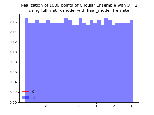
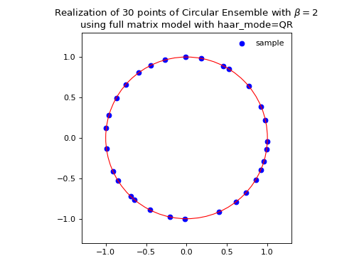
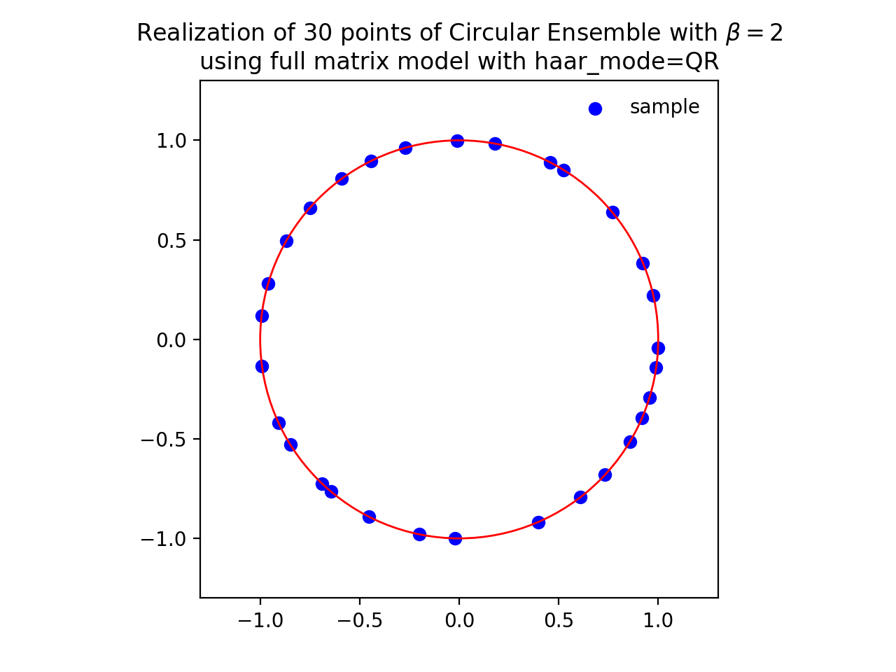
Circular Ensemble
Hint
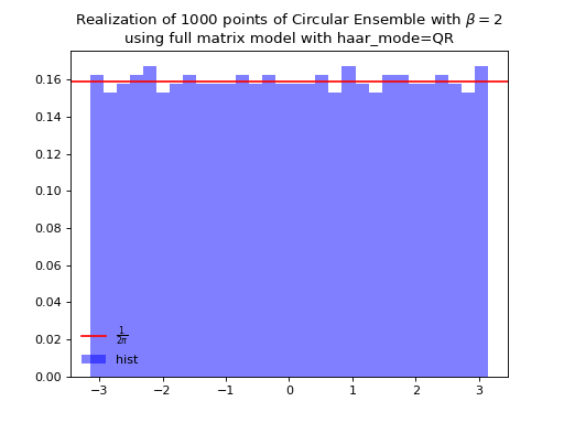
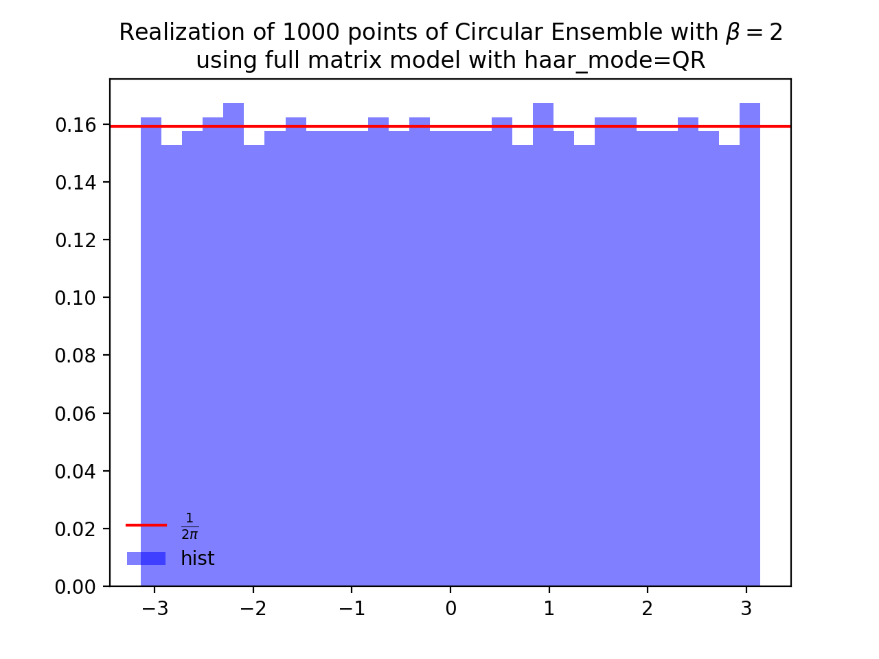
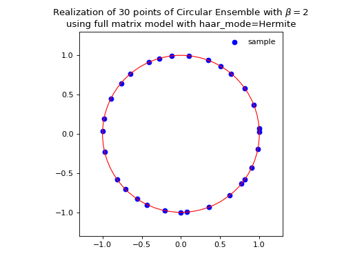
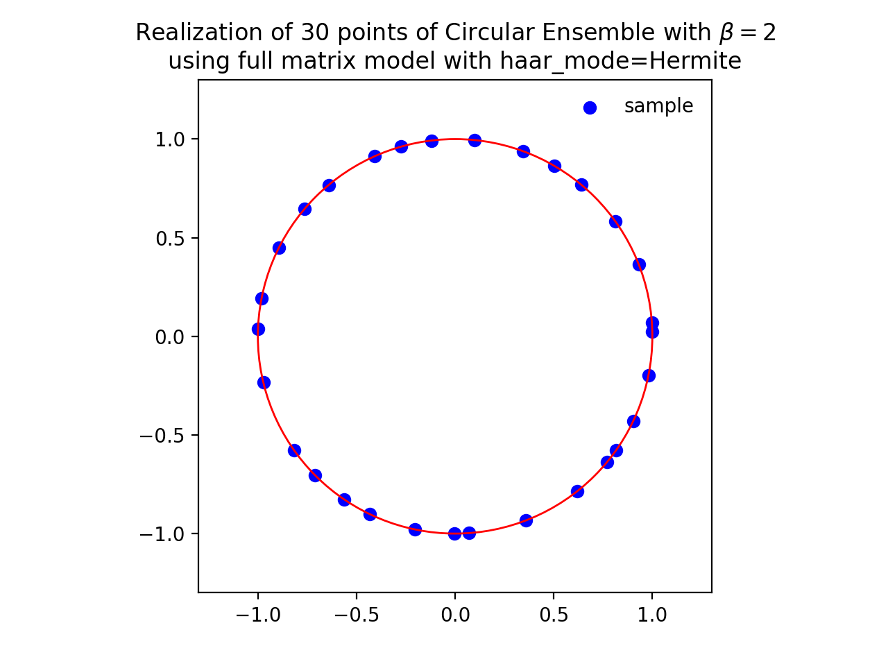
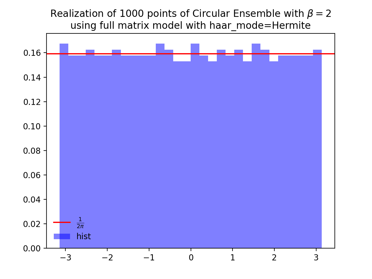
Eigenvalues of orthogonal (resp. unitary and self-dual unitary) matrices drawn uniformly i.e. Haar measure on the respective groups. The eigenvalues lie on the unit circle i.e. \(\lambda_n = e^{i \theta_n}\). The distribution of the angles \(\theta_n\) converges to the uniform measure on \([0, 2\pi[\) as \(N\) grows.
\(\beta=1\)
Uniform measure i.e. Haar measure on orthogonal matrices \(\mathbb{O}_N\): \(U^{\top}U = I_N\)
Via QR algorithm, see [Mez06] Section 5
import numpy as np
from numpy.random import randn
import scipy.linalg as la

A = randn(N, N)
Q, R = la.qr(A)
d = np.diagonal(R)
U = np.multiply(Q, d/np.abs(d), Q)
la.eigvals(U)
The Hermite way
\[\begin{split} X \sim \mathcal{N}_{N, N}(0,1)\\ A = X+X^{\top} = U^{\top}\Lambda U\\ eigvals(U).\end{split}\]\(\beta=2\)
Uniform measure i.e. Haar measure on unitary matrices \(\mathbb{U}_N\): \(U^{\dagger}U = I_N\)
Via QR algorithm, see [Mez06] Section 5
import numpy as np
from numpy.random import randn
import scipy.linalg as la

A = randn(N, N) + 1j*randn(N, N)
Q, R = la.qr(A)
d = np.diagonal(R)
U = np.multiply(Q, d / np.abs(d), Q)
la.eigvals(U)
from dppy.beta_ensembles import CircularEnsemble

circular = CircularEnsemble(beta=2)  # beta in {0,1,2,4}, default beta=2

# 1. Plot the eigenvalues, they lie on the unit circle
circular.sample_full_model(size_N=30, haar_mode='QR')
circular.plot()

# 2. Histogram of the angle of more points, should look uniform on [0,2pi]
circular.flush_samples()  # Flush previous sample

circular.sample_full_model(size_N=1000, haar_mode='QR')
circular.hist()

Fig. 14 (png, hires.png, pdf) Full matrix model for the Circular ensemble from QR on random Gaussian matrix

Fig. 15 (png, hires.png, pdf) Full matrix model for the Circular ensemble from QR on random Gaussian matrix
The Hermite way
\[\begin{split} X \sim \mathcal{N}_{N, N}(0,1) + i~ \mathcal{N}_{N, N}(0,1)\\ A = X+X^{\dagger} = U^{\dagger}\Lambda U\\ eigvals(U).\end{split}\]from dppy.beta_ensembles import CircularEnsemble circular = CircularEnsemble(beta=2) # beta in {0,1,2,4}, default beta=2 # 1. Plot the eigenvalues, they lie on the unit circle circular.sample_full_model(size_N=30, haar_mode='Hermite') circular.plot() # 2. Histogram of the angle of more points, should look uniform on [0,2pi] circular.flush_samples() # Flush previous sample circular.sample_full_model(size_N=1000, haar_mode='Hermite') circular.hist()
\(\beta=4\)
Uniform measure i.e. Haar measure on self-dual unitary matrices \(\mathbb{U}\operatorname{Sp}_{2N}\): \(U^{\dagger}U = I_{2N}\)
\[\begin{split} \begin{cases} X \sim \mathcal{N}_{N, M}(0,1) + i~ \mathcal{N}_{N, M}(0,1)\\ Y \sim \mathcal{N}_{N, M}(0,1) + i~ \mathcal{N}_{N, M}(0,1) \end{cases}\\ A = \begin{bmatrix} X & Y \\ -Y^* & X^* \end{bmatrix} \quad A = X+X^{\dagger} = U^{\dagger} \Lambda U\\ eigvals(U).\end{split}\]

See also
Banded matrix model for Circular ensemble
CircularEnsemblein API
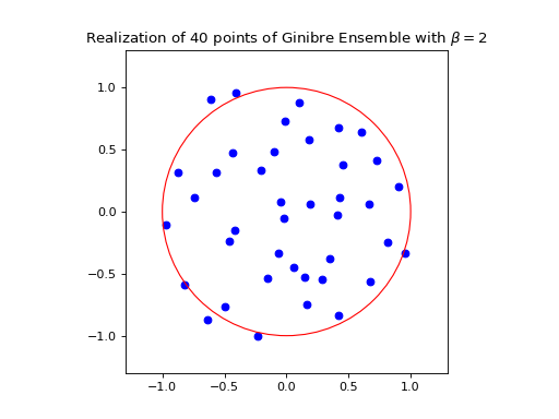
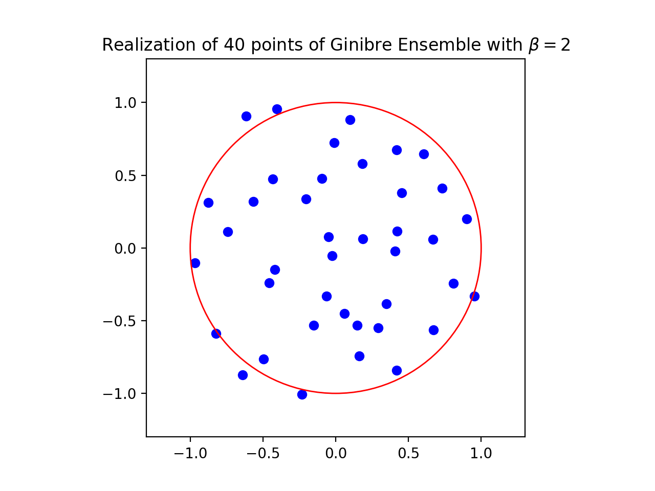
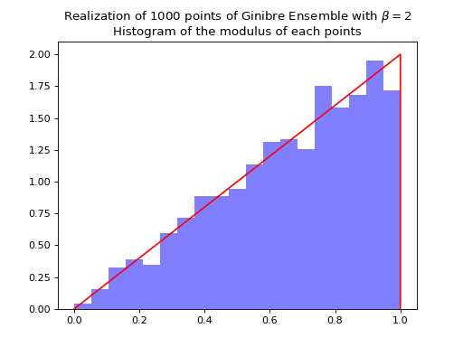
Ginibre Ensemble
where from the definition in (33) we have \(\left|\Delta(x_1,\dots,x_N)\right| = \prod_{i<j} |x_i - x_j|\).
Nomalization \(\sqrt{N}\) to concentrate in the unit circle.
from dppy.beta_ensembles import GinibreEnsemble


ginibre = GinibreEnsemble()  # beta must be 2 (default)

ginibre.sample_full_model(size_N=40)
ginibre.plot(normalization=True)

ginibre.sample_full_model(size_N=1000)
ginibre.hist(normalization=True)

See also
GinibreEnsemblein API