Definition
A finite point process \(\mathcal{X}\) on \([N] \triangleq \{1,\dots,N\}\) can be understood as a random subset. It is defined either via its:
inclusion probabilities (also called correlation functions)
\[\mathbb{P}[S\subset \mathcal{X}], \text{ for } S\subset [N],\]likelihood
\[\mathbb{P}[\mathcal{X}=S], \text{ for } S\subset [N].\]
Hint
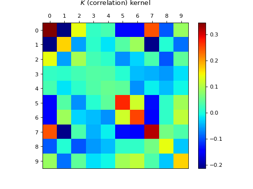
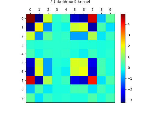
The determinantal feature of DPPs stems from the fact that such inclusion, resp. marginal probabilities are given by the principal minors of the corresponding correlation kernel \(\mathbf{K}\) (resp. likelihood kernel \(\mathbf{L}\)).
Inclusion probabilities
We say that \(\mathcal{X} \sim \operatorname{DPP}(\mathbf{K})\) with correlation kernel a complex matrix \(\mathbf{K}\) if
(1)¶\[\mathbb{P}[S\subset \mathcal{X}] = \det \mathbf{K}_S, \quad \forall S\subset [N],\]
where \(\mathbf{K}_S = [\mathbf{K}_{ij}]_{i,j\in S}\) i.e. the square submatrix of \(\mathbf{K}\) obtained by keeping only rows and columns indexed by \(S\).
Likelihood
We say that \(\mathcal{X} \sim \operatorname{DPP}(\mathbf{L})\) with likelihood kernel a complex matrix \(\mathbf{L}\) if
Existence
Some common sufficient conditions to guarantee existence are:
where the dagger \(\dagger\) symbol means conjugate transpose.
Note
In the following, unless otherwise specified:
# from numpy import sqrt
from numpy.random import rand, randn
from scipy.linalg import qr
from dppy.finite_dpps import FiniteDPP

r, N = 4, 10
e_vecs, _ = qr(randn(N, r), mode='economic')

# Inclusion K
e_vals_K = rand(r)  # in [0, 1]
dpp_K = FiniteDPP('correlation', **{'K_eig_dec': (e_vals_K, e_vecs)})
# or
# K = (e_vecs * e_vals_K).dot(e_vecs.T)
# dpp_K = FiniteDPP('correlation', **{'K': K})
dpp_K.plot_kernel()

# Marginal L
e_vals_L = e_vals_K / (1.0 - e_vals_K)
dpp_L = FiniteDPP('likelihood', **{'L_eig_dec': (e_vals_L, e_vecs)})
# or
# L = (e_vecs * e_vals_L).dot(e_vecs.T)
# dpp_L = FiniteDPP('likelihood', **{'L': K})
# Phi = (e_vecs * sqrt(e_vals_L)).T
# dpp_L = FiniteDPP('likelihood', **{'L_gram_factor': Phi})  # L = Phi.T Phi
dpp_L.plot_kernel()


Projection DPPs
Important
\(\operatorname{DPP}(\mathbf{K})\) defined by an orthogonal projection correlation kernel \(\mathbf{K}\) are called projection DPPs.
Recall that orthogonal projection matrices are notably characterized by
\(\mathbf{K}^2=\mathbf{K}\) and \(\mathbf{K}^{\dagger}=\mathbf{K}\),
or equivalently by \(\mathbf{K}=U U^{\dagger}\) with \(U^{\dagger} U=I_r\) where \(r=\operatorname{rank}(\mathbf{K})\).
They are indeed valid kernels since they meet the above sufficient conditions: they are Hermitian with eigenvalues \(0\) or \(1\).
from numpy import ones
from numpy.random import randn
from scipy.linalg import qr
from dppy.finite_dpps import FiniteDPP

r, N = 4, 10

eig_vals = ones(r)
A = randn(r, N)
eig_vecs, _ = qr(A.T, mode='economic')

proj_DPP = FiniteDPP('correlation', projection=True,
                     **{'K_eig_dec': (eig_vals, eig_vecs)})
# or
# proj_DPP = FiniteDPP('correlation', projection=True, **{'A_zono': A})
# K = eig_vecs.dot(eig_vecs.T)
# proj_DPP = FiniteDPP('correlation', projection=True, **{'K': K})
k-DPPs
A \(k\!\operatorname{-DPP}\) can be defined as \(\operatorname{DPP(\mathbf{L})}\) (2) conditioned to a fixed sample size \(|\mathcal{X}|=k\), we denote it \(k\!\operatorname{-DPP}(\mathbf{L})\).
It is naturally defined through its joint probabilities
where the normalizing constant \(e_k(L)\) corresponds to the elementary symmetric polynomial of order \(k\) evaluated in the eigenvalues of \(\mathbf{L}\),
Note
Obviously, one must take \(k \leq \operatorname{rank}(L)\) otherwise \(\det \mathbf{L}_S = 0\) for \(|S| = k > \operatorname{rank}(L)\).
Warning
k-DPPs are not DPPs in general. Viewed as a \(\operatorname{DPP}\) conditioned to a fixed sample size \(|\mathcal{X}|=k\), the only case where they coincide is when the original DPP is a projection \(\operatorname{DPP}(\mathbf{K})\), and \(k=\operatorname{rank}(\mathbf{K})\), see (13).